Optimizing Matrix Multiplication
Matrix multiplication is an incredibly common operation across numerous domains. It is also known as being “embarrassingly parallel”. As such, one common optimization is parallelization across threads on a multi-core CPU or GPU. However, parallelization is not a panacea. Poorly parallelized code may provide minimal speedups (if any).
In this blog post, we’ll be comparing a few different implementations of matrix multiplication, and show how we can get significant performance improvement from both restructuring access patterns and parallelization.
Links
- These Benchmarks on GitHub
- My YouTube Channel
- My GitHub Account
- My Email: CoffeeBeforeArch@gmail.com
My Testing Environment
The results in this blog post were collected on my home desktop running Ubuntu 20.04, with an 8 core Intel Core i7-9700 processor. All benchmarks were written using Google Benchmark, and hotspot/performance counter information was collected using the perf Linux profiler.
The benchmarks can be found in the gemm repo on my GitHub page. GEMM (generalized matrix multiplication) includes the scaling of our A matrix by some constant (alpha), and the addition of the C matrix multiplied by some constant (beta). For these benchmarks, we’ll be just looking at the core matrix multiplication component, and assume alpha is 1, and beta is 0 for all cases.
There is a simple Makefile in the src directory that can be used to build the benchmarks. The benchmarks are compiled using the following flags:
CXX_FLAGS = -O3 -march=native -mtune=native -flto -fuse-linker-plugin --std=c++2a
It also requires you to use the linker flags -lbenchmark and -lpthread (both of which are required for Google Benchmark).
Matrix Multiplication - Baseline
Let’s look at an implementation of matrix multiplication that will likely be familiar to many of you.
void serial_gemm(const double *A, const double *B, double *C, std::size_t N) {
  // For each row...
  for (std::size_t row = 0; row < N; row++)
    // For each col...
    for (std::size_t col = 0; col < N; col++)
      // For each element in the row/col pair...
      for (std::size_t idx = 0; idx < N; idx++)
        // Accumulate the partial results
        C[row * N + col] += A[row * N + idx] * B[idx * N + col];
}
Let’s break down this function loop-by-loop to understand how we are traversing the A, B, and C matrices (something we will do for each of these examples).
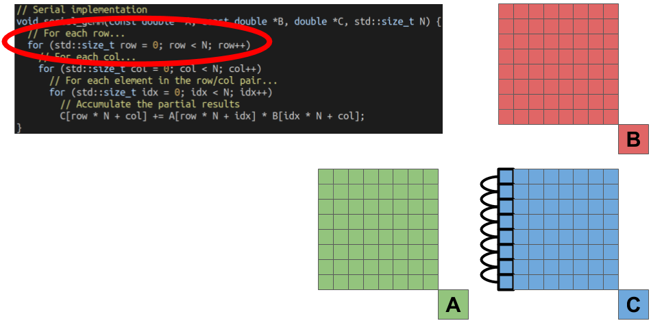
The outermost-loop of the function selects the row of the element we are going to solve for.
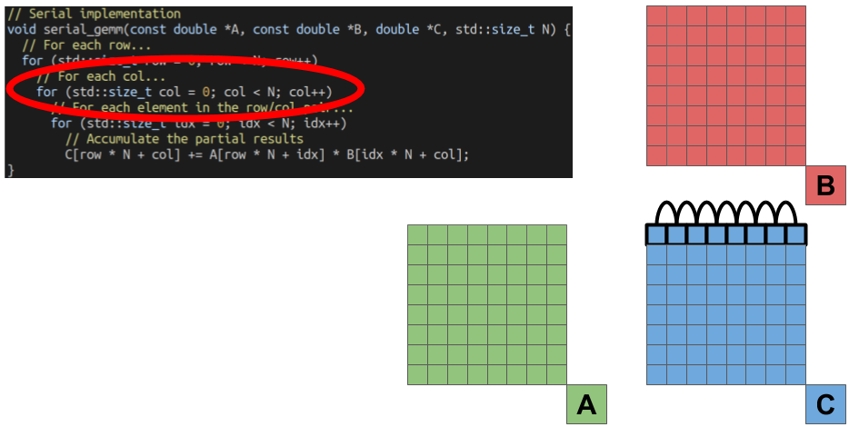
The next loop then selects the column of the element we are solving for.
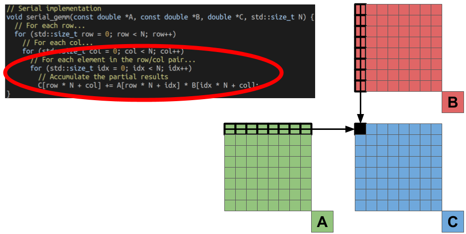
The combination of the row and column index gives us the coordinate of a single element in the output matrix C we are solving for. The final, inner-most loop performs this computation by doing the dot-product of one Row of the A matrix by one column of the B matrix.
Computationally, how much work are we doing? For the square matrices of dimension NxN we are working with, we perform N multiplies and adds for the dot product of each output element. This results in N^3 FMA (fused multiply-add) operations.
Now that we understand the computational complexity of this algorithm, let’s take a look at some initial performance numbers. Let’s test our serial gemm function for square matrix sizes of 2^8, 2^9, and 2^10. Here are the results.
Benchmark                               Time             CPU   Iterations
-------------------------------------------------------------------------
serial_gemm_bench_power_two/8        21.9 ms         21.9 ms           64
serial_gemm_bench_power_two/9         177 ms          177 ms            8
serial_gemm_bench_power_two/10       2039 ms         2039 ms            1
Pretty slow for the 2^10 case. However, we are running into a rather nasty performance corner case using power-of-two dimension matrices. Each access we make to our B matrix is 2^N elements apart. Having an access pattern with this kind of stride can lead to many conflict misses, as each cache line will be mapped to a small subset of cache sets (or even a single cache set).
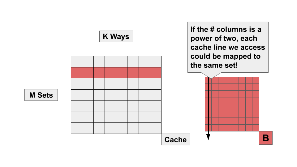
Each set has a limited number of ways (usually something like 4 or 8). While the size of our cache (in bytes) may be relatively large compared to the size of our matrices, we can’t make effective use of this capacity if every cache line is fighting for the same 4 or 8 ways in a single set. Let’s try slightly increasing the size of our matrix, and re-collect the performance numbers. We’ll use 2^8 + 16, 2^9 + 16, and 2^10 + 16. Here are the performance numbers:
---------------------------------------------------------------
Benchmark                     Time             CPU   Iterations
---------------------------------------------------------------
serial_gemm_bench/8        16.2 ms         16.2 ms           85
serial_gemm_bench/9         126 ms          126 ms           11
serial_gemm_bench/10       1067 ms         1067 ms            1
Despite doing more work, our performance improves (and by a fairly large margin!). We’ll use these augmented sizes (2^8 + 16, 2^9 + 16, and 2^10 + 16) for the rest of our experiments.
But first, what is going on in our assembly? Here’s a look at the hotspot of our serial implementation.
  0.40 │2b8:┌─→vmovsd      (%rax),%xmm1
 23.40 │    │  add         $0x8,%rax
 74.88 │    │  vfmadd231sd (%rdx),%xmm1,%xmm0
  0.42 │    │  add         %rbx,%rdx
       │    ├──cmp         %rax,%rcx
  0.44 │    └──jne         2b8
All of our time is being spend around a single FMA (fused multiply-add) instruction! We’re processing one output element at a time in our inner loop (for better or worse).
Matrix Multiplication - Parallel
Now that we have our baseline performance numbers, let’s see if we can get some extra performance from parallelization. Here is how my implementation looks.
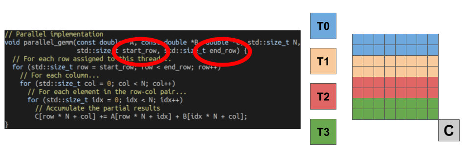
// Parallel implementation
void parallel_gemm(const double *A, const double *B, double *C, std::size_t N,
                   std::size_t start_row, std::size_t end_row) {
  // For each row assigned to this thread...
  for (std::size_t row = start_row; row < end_row; row++)
    // For each column...
    for (std::size_t col = 0; col < N; col++)
      // For each element in the row-col pair...
      for (std::size_t idx = 0; idx < N; idx++)
        // Accumulate the partial results
        C[row * N + col] += A[row * N + idx] * B[idx * N + col];
We can divide up the work by dividing the mapping rows of the output matrix to different threads. The only change I’ve made to the original serial code is passing in the start row and end row to the function. Here is a figure on how we have divided up the work.
Assuming we can divide our matrix evenly by the number of threads we launch (assumed to be true), each thread performs the same ammount of work. Let’s check out how our performance improved (we’ll look at the Time column numbers for multi-threaded benchmarks, which reports the wall-clock time).
---------------------------------------------------------------------------
Benchmark                                 Time             CPU   Iterations
---------------------------------------------------------------------------
parallel_gemm_bench/8/real_time        2.46 ms         2.42 ms          579
parallel_gemm_bench/9/real_time        17.5 ms         17.4 ms           78
parallel_gemm_bench/10/real_time        152 ms          152 ms            9
A huge improvement! For our largest matrix size (2^10 + 16), we’ve improved execution time from ~1000ms to ~150ms. That’s a huge improvement for minimal changes to our original function (plus a few extra lines for spawning/joining threads). However, we’re far from done with this example.
Matrix Multiplication - Blocked
Let’s see if we can be a little more clever about the order in which we process elements. Specifically, let’s begin to focus on exploiting locality in the B matrix. In our serial benchmark, we access one element from each row of the B matrix (from Row 0 -> N-1). However, that’s not what our processor is doing under the hood. When we access a single element from B, our processor loads the entire cache line that element is sitting on into the cache. Most processors have a 64B cache line, which can fit at most 16 ints/float, or 8 doubles.
If we only access a single element from each row of the B matrix at a time, we’re wasting the other sitting on that cache line if we do not use them. Furthermore, by the time we get back around to accessing the other elements, they may have already been replaced in the cache. Instead of processing a single element at a time, let’s process an entire block of elements so that we use these extra elements loaded in from the B matrix (this optimization is often called blocking or tiling). Here is my code.
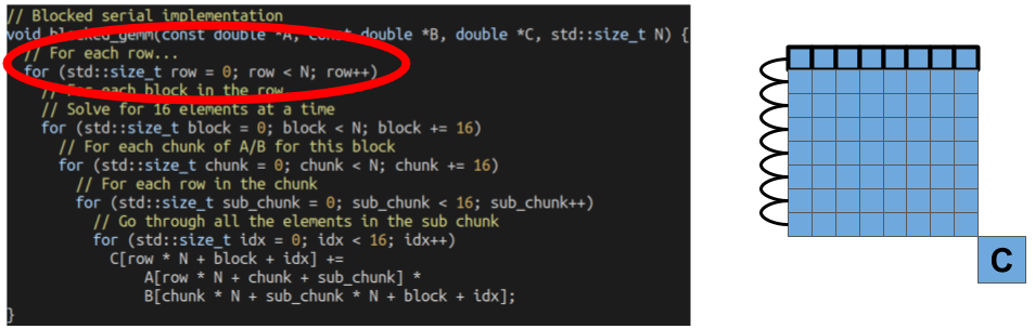
// Blocked serial implementation
void blocked_gemm(const double *A, const double *B, double *C, std::size_t N) {
// For each row...
for (std::size_t row = 0; row < N; row++)
// For each block in the row...
// Solve for 16 elements at a time
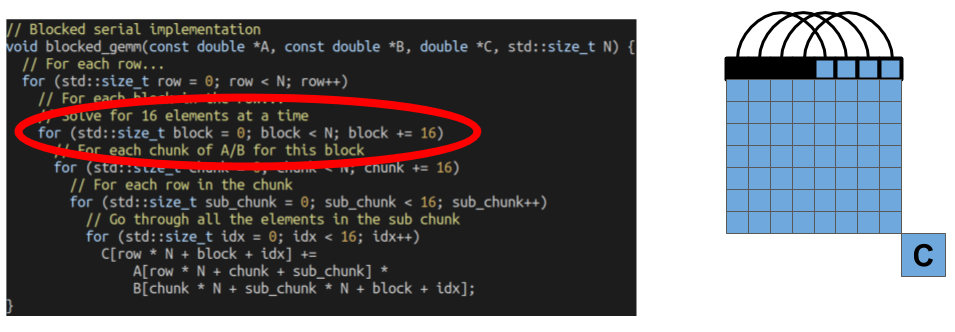
for (std::size_t block = 0; block < N; block += 16)
// For each chunk of A/B for this block
for (std::size_t chunk = 0; chunk < N; chunk += 16)
// For each row in the chunk
for (std::size_t sub_chunk = 0; sub_chunk < 16; sub_chunk++)
// Go through all the elements in the sub chunk
for (std::size_t idx = 0; idx < 16; idx++)
C[row * N + block + idx] +=
A[row * N + chunk + sub_chunk] *
B[chunk * N + sub_chunk * N + block + idx];
}
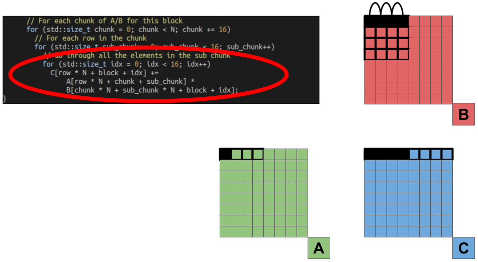
All we’ve done is added a few extra loops to handle the blocking/tiling. Let’s take a look at how we’ve decomposed the computation into blocks.
We can start with the outer-most loop. We’re processing output elements of the C matrix one row at a time (the same as our serial implementation).
However, our next loop is where we change things up. Instead of processing elements one column at a time, we’re going to process elements a block at a time. This will allow us to re-use elements loaded from the B matrix.
For each block of elements we are solving for, our next loop processes elements from the A and B matrices one chunk at a time. Since we’re not processing the entirety of these matrices at once, the pieces are more likely to fit into our caches.
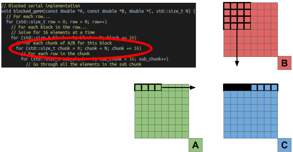
The next loop is for processing elements from each chunk (we’ll call it a sub chunk). We’ll go through each row of the chunk of the B matrix, and each element from the chunk of the A matrix.
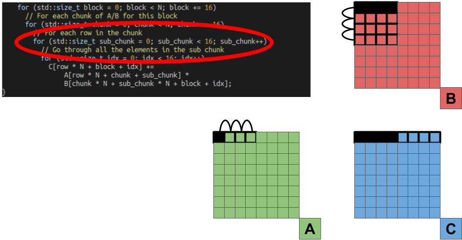
The final loop is for actually performing the computation (yay, we made it!). In this loop, we multiply the elements of the B matrix by one of the elements of the A matrix, and storing the partial results in the result block of elements from the C matrix.
 .
.
Now that we have some understanding of what the loops are doing, let’s look at the performance results.
-----------------------------------------------------------------------------------
Benchmark                                         Time             CPU   Iterations
-----------------------------------------------------------------------------------
blocked_gemm_bench/8                           4.72 ms         4.72 ms          300
blocked_gemm_bench/9                           36.8 ms         36.8 ms           38
blocked_gemm_bench/10                           386 ms          386 ms            4
Impressive results! We’re getting close to the speed of our parallelized version with just a single thread (~150ms vs ~390ms on the largest matrix size).
However, we’re not quite done with our blocked version yet. Our performance is based on our assumption about exploiting locality. To help out with this, we can use something like aligned_alloc instead of new to have the memory for our matrix be aligned to the start of a cache line. While this isn’t guaranteed to help performance, it can be especially useful where we’re making assumptions about locality, and what elements should be sitting on the same cache line. Here are the performance results when using aligned_alloc instead of new for our matrices.
Benchmark                              Time             CPU   Iterations
------------------------------------------------------------------------
blocked_aligned_gemm_bench/8        3.50 ms         3.50 ms          398
blocked_aligned_gemm_bench/9        28.2 ms         28.2 ms           50
blocked_aligned_gemm_bench/10        309 ms          309 ms            4
A fairly substantial improvement! Now let’s look at the assembly.
  0.23 │     → jmp          afcb <blocked_gemm(double const*, double cons▒
       │       nop                                                       ▒
  1.13 │       mov          %rax,%rdi                                    ▒
  0.66 │       sub          %rdx,%rdi                                    ▒
  3.05 │       cmp          $0x10,%rdi                                   ▒
       │     → jbe          afe5 <blocked_gemm(double const*, double cons▒
  1.98 │       vbroadcastsd (%rcx),%ymm0                                 ▒
 12.59 │       vmovupd      -0x8(%rdx),%ymm1                             ▒
  1.90 │       vmovupd      0x60(%rax),%ymm2                             ▒
  9.71 │       vfmadd213pd  (%rax),%ymm0,%ymm1                           ▒
  3.18 │       vmovupd      %ymm1,(%rax)                                 ▒
  2.10 │       vmovupd      0x18(%rdx),%ymm1                             ▒
  8.24 │       vfmadd213pd  0x20(%rax),%ymm0,%ymm1                       ▒
  3.84 │       vmovupd      %ymm1,0x20(%rax)                             ▒
  9.32 │       vmovupd      0x38(%rdx),%ymm1                             ▒
  8.65 │       vfmadd213pd  0x40(%rax),%ymm0,%ymm1                       ▒
  2.90 │       vmovupd      %ymm1,0x40(%rax)                             ▒
 12.14 │       vfmadd132pd  0x58(%rdx),%ymm2,%ymm0                       ▒
  0.61 │       add          %r11,%rdx                                    ▒
  2.90 │       vmovupd      %ymm0,0x60(%rax)                             ◆
  1.36 │       cmp          %rsi,%r9                                     ▒
  0.12 │     → je           b12e <blocked_gemm(double const*, double cons▒
  1.34 │       mov          %rsi,%rcx                                    ▒
  0.65 │       add          $0x8,%rsi                                    ▒
  2.69 │       cmp          %r10,%rcx                                    ▒
  1.78 │       setae        %r8b                                         ▒
  1.37 │       cmp          %rsi,%rax                                    ▒
  0.61 │       setae        %dil                                         ▒
  2.59 │       or           %dil,%r8b                                    ▒
  1.69 │     → jne          af70 <blocked_gemm(double const*, double cons▒
Instead of processing a single element at a time (like we saw in our baseline code), we’re working on multiple! We’re able to do far more work in our inner loops by processing elements that are spatially close to each other!
Matrix Multiplication - Blocked + Parallel
We can parallelize our our blocked implementation the same way we parallelized our original serial implementation. Here is how my implementation looks.
// Blocked parallel implementation
void blocked_parallel_gemm(const double *A, const double *B, double *C,
                           std::size_t N, std::size_t start_row,
                           std::size_t end_row) {
  // For each row...
  for (std::size_t row = start_row; row < end_row; row++)
    // For each block in the row...
    // Solve for 16 elements at a time
    for (std::size_t block = 0; block < N; block += 16)
      // For each chunk of A/B for this block
      for (std::size_t chunk = 0; chunk < N; chunk += 16)
        // For each row in the chunk
        for (std::size_t sub_chunk = 0; sub_chunk < 16; sub_chunk++)
          // Go through all the elements in the sub chunk
          for (std::size_t idx = 0; idx < 16; idx++)
            C[row * N + block + idx] +=
                A[row * N + chunk + sub_chunk] *
                B[chunk * N + sub_chunk * N + block + idx];
}
Just like our previous parallel implementation, we’ve mapped slices of rows to different threads. The only change I’ve made to the original blocked code is passing in the start row and end row to the function. Here is figure of how we have divided up the work.
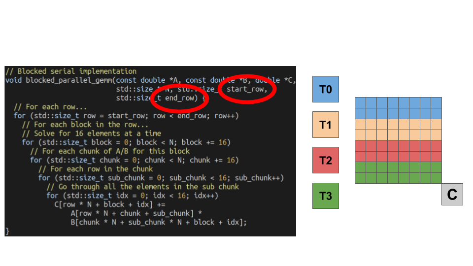
Assuming we can divide our matrix evenly by the number of threads we launch (assumed to be true), each thread performs the same ammount of work. Let’s check out how our performance improved (we’ll look at the Time column numbers for multi-threaded benchmarks which reports the wall-clock time).
-----------------------------------------------------------------------------------
Benchmark                                         Time             CPU   Iterations
-----------------------------------------------------------------------------------
parallel_blocked_gemm_bench/8/real_time        1.57 ms        0.685 ms         1078
parallel_blocked_gemm_bench/9/real_time        8.02 ms         4.32 ms          188
parallel_blocked_gemm_bench/10/real_time        107 ms         46.4 ms           16
A decent bit faster than our original parallel implementation and serial blocked implementation. Don’t worry, we’re not done yet! There’s still more locality we’re not exploiting!
Matrix Multiplication - Blocked-Column
One way of blocking is across a row of the C matrix (what we just did). However, this does a lot of wasted work. Whenever we move to a new block, we access a completely new set of columns from the B matrix, and re-use a single row of the A matrix. This means we access the entirety of the B matrix multiple times. Instead, let’s re-use the columns of B, instead of a single row of A. Here is my implementation of a blocked-column algorithm:
// Blocked serial implementation
void blocked_column_gemm(const double *A, const double *B, double *C,
                         std::size_t N) {
  // For each chunk of columns
  for (std::size_t col_chunk = 0; col_chunk < N; col_chunk += 16)
    // For each row in that chunk of columns...
    for (std::size_t row = 0; row < N; row++)
      // For each block of elements in this row of this column chunk
      // Solve for 16 elements at a time
      for (std::size_t tile = 0; tile < N; tile += 16)
        // For each row in the tile
        for (std::size_t tile_row = 0; tile_row < 16; tile_row++)
          // Solve for each element in this tile row
          for (std::size_t idx = 0; idx < 16; idx++)
            C[row * N + col_chunk + idx] +=
                A[row * N + tile + tile_row] *
                B[tile * N + tile_row * N + col_chunk + idx];
}
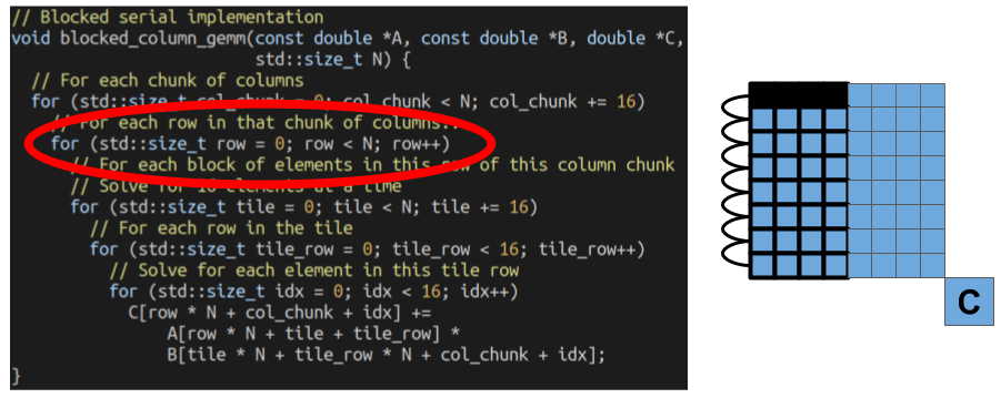
The outermost loop select which columns of elements we are going to solve from the C matrix.
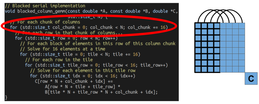
Then, we go through all the rows inside of that column chunk. All the elements of these rows will re-use the same columns from the B matrix. We’re aiming at exploiting the localitiy within a single column chunk with this optimization.
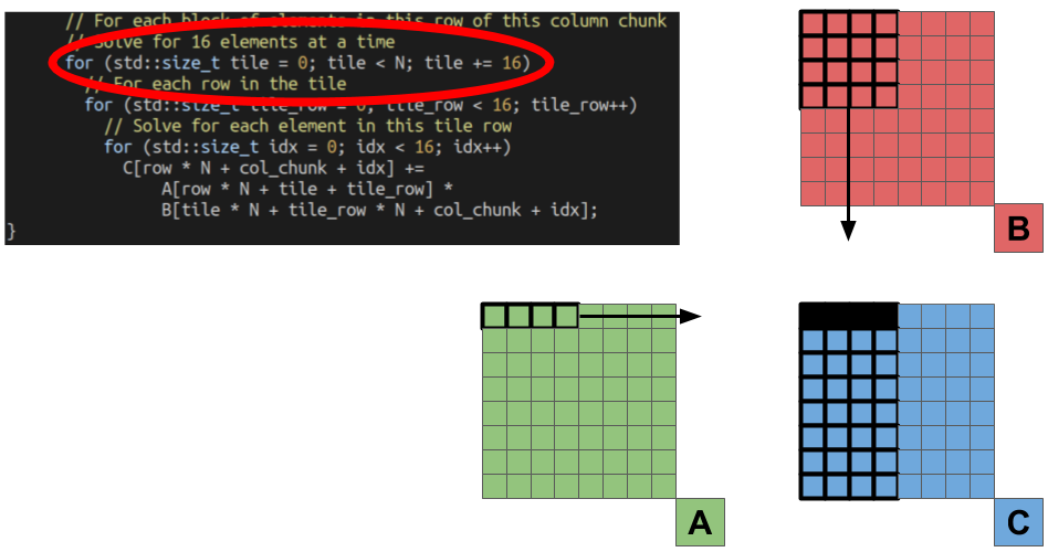
From there, the process is exactly the same as our original blocked algorithm. We start by only processing one tile of elements from matrices A and B.
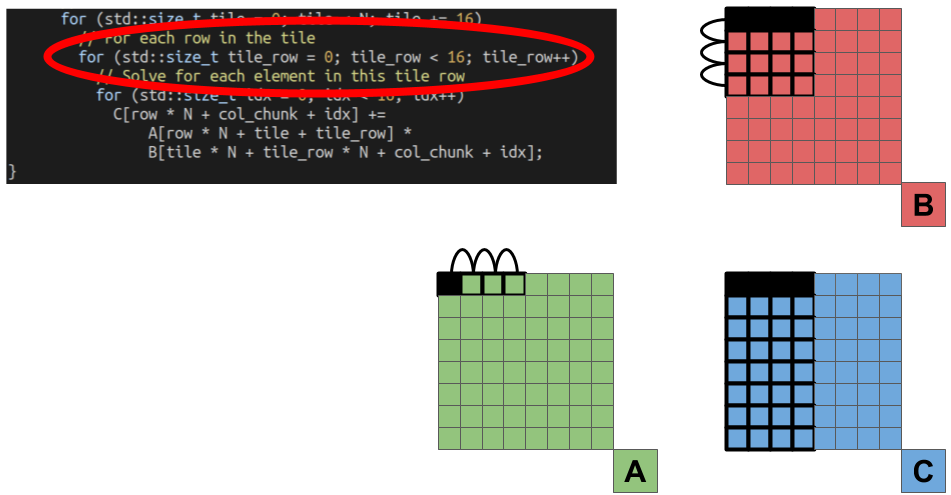
For each tile, we then have to go through all the rows of the B tile, and the coulmns of the A tile.
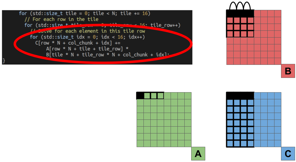
Finally, we multiply each element in the row of the B matrix tile, with a single element from the A matrix tile, and accumulate the partial results into the results stored in the C matrix.
Now that we understand the algorithm let’s look at the performance numbers:
-------------------------------------------------------------------------------
Benchmark                                     Time             CPU   Iterations
-------------------------------------------------------------------------------
blocked_column_aligned_gemm_bench/8        1.80 ms         1.80 ms          772
blocked_column_aligned_gemm_bench/9        14.5 ms         14.5 ms           95
blocked_column_aligned_gemm_bench/10        138 ms          138 ms           10
We now have a single-threaded version that is faster than our baseline parallel implementation for all cases! We’re also fairly close to our blocked + parallel performance! Now let’s look at the assembly.
  0.29 │2ec:┌─→lea          (%rsi,%rdi,1),%rcx                                           ▒
  0.18 │    │  mov          %rsi,%rdx                                                    ▒
  0.19 │    │  xor          %r10d,%r10d                                                  ▒
  4.92 │2f6:│  vbroadcastsd (%r8,%r10,8),%ymm1                                           ▒
  1.21 │    │  vbroadcastsd 0x8(%r8,%r10,8),%ymm5                                        ▒
  9.89 │    │  vfmadd231pd  (%rdx),%ymm1,%ymm4                                           ▒
  6.19 │    │  vfmadd231pd  0x20(%rdx),%ymm1,%ymm3                                       ▒
  6.78 │    │  vfmadd231pd  0x40(%rdx),%ymm1,%ymm2                                       ▒
  4.35 │    │  vfmadd231pd  0x60(%rdx),%ymm1,%ymm0                                       ▒
  1.03 │    │  add          $0x2,%r10                                                    ▒
 14.03 │    │  vfmadd231pd  (%rcx),%ymm5,%ymm4                                           ▒
  8.58 │    │  vfmadd231pd  0x20(%rcx),%ymm5,%ymm3                                       ▒
  8.03 │    │  vfmadd231pd  0x40(%rcx),%ymm5,%ymm2                                       ▒
  5.76 │    │  vfmadd231pd  0x60(%rcx),%ymm5,%ymm0                                       ▒
  1.07 │    │  add          %r11,%rdx                                                    ▒
  1.33 │    │  vmovupd      %ymm4,(%rax)                                                 ▒
  1.74 │    │  vmovupd      %ymm3,0x20(%rax)                                             ▒
  2.08 │    │  vmovupd      %ymm2,0x40(%rax)                                             ▒
  1.04 │    │  vmovupd      %ymm0,0x60(%rax)                                             ▒
  1.22 │    │  add          %r11,%rcx                                                    ▒
  0.24 │    │  cmp          $0xe,%r10                                                    ▒
  1.33 │    │↑ jne          2f6                                                          ▒
  0.28 │    │  mov          0x20(%rsp),%rdx                                              ▒
  0.08 │    │  lea          0x70(%r8),%rcx                                               ▒
  0.15 │    │  add          %rsi,%rdx                                                    ▒
  0.28 │    │  sub          $0xffffffffffffff80,%r8                                      ▒
  0.53 │364:│  vbroadcastsd (%rcx),%ymm1                                                 ▒
  0.34 │    │  add          $0x8,%rcx                                                    ▒
  5.32 │    │  vfmadd231pd  (%rdx),%ymm1,%ymm4                                           ▒
  2.67 │    │  vfmadd231pd  0x20(%rdx),%ymm1,%ymm3                                       ▒
  1.79 │    │  vfmadd231pd  0x40(%rdx),%ymm1,%ymm2                                       ▒
  1.47 │    │  vfmadd231pd  0x60(%rdx),%ymm1,%ymm0                                       ▒
  0.26 │    │  add          %rdi,%rdx                                                    ▒
  0.43 │    │  vmovupd      %ymm4,(%rax)                                                 ▒
  0.48 │    │  vmovupd      %ymm3,0x20(%rax)                                             ▒
  0.58 │    │  vmovupd      %ymm2,0x40(%rax)                                             ▒
  0.29 │    │  vmovupd      %ymm0,0x60(%rax)                                             ▒
  0.17 │    │  cmp          %r8,%rcx                                                     ▒
  0.19 │    │↑ jne          364                                                          ▒
  0.23 │    │  add          $0x10,%r9                                                    ◆
  0.33 │    │  add          %r13,%rsi                                                    ▒
  0.22 │    │  cmp          %r9,%rbx                                                     ▒
       │    │↓ jbe          3b3                                                          ▒
  0.15 │    │  mov          %rcx,%r8                                                     ▒
  0.26 │    └──jmpq         2ec                                                          ▒
Slightly different than our original blocked implementation now that we are traversing down the column of our output matrix. However, we are similarly processing more than a single element at a time in the iterations of our inner loop!
If we can process matrices this quickly with just a single thread, what happens when we parallelize our blocked-column algorithm?
Matrix Multiplication - Blocked-Column + Parallel
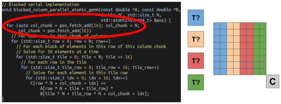
Let’s parallelize our blocked-column algorithm! However, we have to decompose our problem slightly differently. Because our algorithm is based around blocks of columns, we have less flexibility in how we divide up our work. This is because the number of columns we give each thread must be a multiple of 16 (because the outer loop increments by 16). However, we can get around this fairly easily by having each thread work on only 16 columns at a time, and come back for more when they are done. Here is that code:
 // Blocked serial implementation
 void blocked_column_parallel_atomic_gemm(const double *A, const double *B,
                                          double *C, std::size_t N,
                                          std::atomic<uint64_t> &pos) {
   for (auto col_chunk = pos.fetch_add(16); col_chunk < N;
        col_chunk = pos.fetch_add(16))
     // For each row in that chunk of columns...
     for (std::size_t row = 0; row < N; row++)
       // For each block of elements in this row of this column chunk
       // Solve for 16 elements at a time
       for (std::size_t tile = 0; tile < N; tile += 16)
         // For each row in the tile
         for (std::size_t tile_row = 0; tile_row < 16; tile_row++)
           // Solve for each element in this tile row
           for (std::size_t idx = 0; idx < 16; idx++)
             C[row * N + col_chunk + idx] +=
                 A[row * N + tile + tile_row] *
                 B[tile * N + tile_row * N + col_chunk + idx];
 }
Each iteration of the outer loop, the starting column number for each thread is given by a call to pos.fetch_add(16). This increments the current global column number by 16, and returns the previous value. While each thread pays the price for finding what chunk of columns they are working on next, this is is relatively small, as it happens only once each iteration of the outermost loop. Furthermore, we it saves us from handling any nasty corner cases in our code.
Here are the performance results (we’ll look at the Time column numbers for multi-threaded benchmarks):
-------------------------------------------------------------------------------------------------
Benchmark                                                       Time             CPU   Iterations
-------------------------------------------------------------------------------------------------
parallel_blocked_column_atomic_gemm_bench/8/real_time       0.614 ms        0.467 ms         2307
parallel_blocked_column_atomic_gemm_bench/9/real_time        3.62 ms         2.97 ms          382
parallel_blocked_column_atomic_gemm_bench/10/real_time       30.0 ms         29.3 ms           46
Our fastest performance numbers yet!
For a fun side project, I manually divided the columns in order to show the overhead without the atomic fetch and add. Here were the results.
------------------------------------------------------------------------------------------
Benchmark                                                Time             CPU   Iterations
------------------------------------------------------------------------------------------
parallel_blocked_column_gemm_bench/8/real_time       0.932 ms        0.317 ms          679
parallel_blocked_column_gemm_bench/9/real_time        3.01 ms        0.881 ms          226
parallel_blocked_column_gemm_bench/10/real_time       14.8 ms         3.03 ms           44
As you can see we get some significant performance improvement for the larger matrix sizes (~2x for the largest size). If we sacrifice some of the generalizability of our implementation, we can almost make things as fast as we want (this is true for most applications)!
Concluding Remarks
Performance does not require everything to be hand-written in assembly, nor does it always require some exceeedingly complex algorithm. Paying attention to what data you are accessing, if/when you are re-accessing it, and finding ways to make best use of this locality can lead to significant performance improvements. Each of our implementations perform N^3 FMA operations. We just changed the order in which these operations were performed.
Even if our problem is “embarrassingly parallel”, that doesn’t mean that parallelism will give us all the performance improvement in the world. With our serial blocked-column algorithm, we were able to process matrices faster than our initial parallel implementation. In many cases, performance is all about the memory! These optimizations are also just a starting point. There are many more optimizations you can perform, especially when you specifically tune your algorithms for the processor you are running on. We were able to get the processing time down from ~1060ms to ~30ms through a just a few optimizations.
As always, feel free to contact me with questions.
Cheers,
–Nick
Links
- These Benchmarks on GitHub
- My YouTube Channel
- My GitHub Account
- My Email: CoffeeBeforeArch@gmail.com